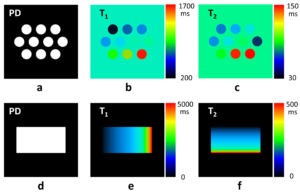
The following images are maps for proton density, T1, and T2 for a relaxation phantom and a dictionary phantom.

 

The relaxation phantom was acquired with the following MR fingerprinting sequence:

from psdk import *
import numpy as np

gamma = 42.57747892 # [MHz/T]
TR = 20.0e+3 # [us]
TE = 4.0e+3 # [us]
NR = 1495 # Number of readout points
NSHOT = 1000 # Number of shots
fov = [256.0, 256.0, 256.0] # [mm]
dwell_time = 5.0 # [us]
slice_width = 6.0 # [mm]
gz_value = 1.25 / (slice_width * 1.0e-3) / gamma # [mT/m]
gx_rise_time = 300.0 # [us]
gy_rise_time = 300.0 # [us]
gz_rise_time = 300.0 # [us]
excitation_pulse_width = 1600.0 # [us]
excitation_pulse_flip_angle = 15.0 # [degree]
gx_waveform = np.fromfile('GX.dbl', dtype=np.float64)
gy_waveform = np.fromfile('GY.dbl', dtype=np.float64)
variable_TR = np.fromfile('Variable_TR.dbl', dtype=np.float64)
variable_FA = np.fromfile('Variable_FA.dbl', dtype=np.float64)

def sinc_with_hamming(flip_angle, pulse_width, points, *, min=-2.0*np.pi, max=2.0*np.pi):
    x0 = np.arange(min, max, (max - min) / points)
    x1 = x0 + (max - min) / points
    y = (np.sinc(x0 / np.pi) + np.sinc(x1 / np.pi)) * 0.5 * np.hamming(points)
    return flip_angle * y * points / (y.sum() * pulse_width * 360.0e-6 * gamma)

with Sequence('2D MRF'):

    with Block('Inversion', excitation_pulse_width):
        RF(0.0, 2.0 * sinc_with_hamming(90.0, excitation_pulse_width, 160), excitation_pulse_width / 160)

    with Block('Excitation', excitation_pulse_width + 2.0*gz_rise_time):
        GZ(0.0, gz_value, gz_rise_time)
        RF(gz_rise_time, sinc_with_hamming(1.0, excitation_pulse_width, 160),
        excitation_pulse_width / 160, factor=(variable_FA, ['SHOT']))
        GZ(excitation_pulse_width + gz_rise_time, 0.0, gz_rise_time)

    with Block("Slice_refocus", excitation_pulse_width * 0.5 + gz_rise_time * 2.0) :
        GZ(0.0, -gz_value, gz_rise_time)
        GZ(excitation_pulse_width * 0.5 + gz_rise_time, 0.0, gz_rise_time) 
        
    with Block('Readout', 10240):
        GX.waveform(0.0, ([gx_waveform[((7*i)%48) * 2048:(((7*i)%48)+1)*2048:] for i in range(NSHOT)], ['SHOT']), 5.0)
        GY.waveform(0.0, ([gy_waveform[((7*i)%48) * 2048:(((7*i)%48)+1)*2048:] for i in range(NSHOT)], ['SHOT']), 5.0)
        AD(0.0, NR, dwell_time)
                
    with Main():
        BlockRef('Inversion')
        WaitUntil(100000)
        with Loop('SHOT', NSHOT):
            BlockRef('Excitation')
            BlockRef('Slice_refocus')
            WaitUntil(TE)
            BlockRef('Readout')
            WaitUntil((variable_TR, ['SHOT']))

 

The dictionary phantom was acquired with the following sequence:

from psdk import *
import numpy as np

gamma = 42.57747892 # [MHz/T]
TR = 20000.0e+3 # [us]
TE = 4.0e+3 # [us]
NR = 1495 # Number of readout points
NSHOT = 1000 # Number of shots
NSHOT1 = 7
fov = [256.0, 256.0, 256.0] # [mm]
dwell_time = 5.0 # [us]
slice_width = 6.0 # [mm]
gz_value = 1.25 / (slice_width * 1.0e-3) / gamma # [mT/m]
gx_rise_time = 300.0 # [us]
gy_rise_time = 300.0 # [us]
gz_rise_time = 300.0 # [us]
excitation_pulse_width = 1600.0 # [us]
excitation_pulse_flip_angle = 15.0 # [degree]
gx_waveform = np.fromfile('GX.dbl', dtype=np.float64)
gy_waveform = np.fromfile('GY.dbl', dtype=np.float64)
variable_TR = np.fromfile('Variable_TR.dbl', dtype=np.float64)
variable_FA = np.fromfile('Variable_FA.dbl', dtype=np.float64)

def sinc_with_hamming(flip_angle, pulse_width, points, *, min=-2.0*np.pi, max=2.0*np.pi):
    x0 = np.arange(min, max, (max - min) / points)
    x1 = x0 + (max - min) / points
    y = (np.sinc(x0 / np.pi) + np.sinc(x1 / np.pi)) * 0.5 * np.hamming(points)
    return flip_angle * y * points / (y.sum() * pulse_width * 360.0e-6 * gamma)

with Sequence('2D MRF'):

    with Block('Inversion', excitation_pulse_width):
        RF(0.0, 2.0 * sinc_with_hamming(90.0, excitation_pulse_width, 160), excitation_pulse_width / 160)

    with Block('Excitation', excitation_pulse_width + 2.0*gz_rise_time):
        GZ(0.0, gz_value, gz_rise_time)
        RF(gz_rise_time, sinc_with_hamming(1.0, excitation_pulse_width, 160),
        excitation_pulse_width / 160, factor=(variable_FA, ['SHOT']))
        GZ(excitation_pulse_width + gz_rise_time, 0.0, gz_rise_time)

    with Block("Slice_refocus", excitation_pulse_width * 0.5 + gz_rise_time * 2.0) :
        GZ(0.0, -gz_value, gz_rise_time)
        GZ(excitation_pulse_width * 0.5 + gz_rise_time, 0.0, gz_rise_time) 
        
    with Block('Readout', 10240):
        GX.waveform(0.0, ([gx_waveform[((7*i+j)%48) * 2048:(((7*i+j)%48)+1)*2048:] for i in range(NSHOT) for j in range(NSHOT1)],
            ['SHOT', 'SHOT1']), 5.0)
        GY.waveform(0.0, ([gy_waveform[((7*i+j)%48) * 2048:(((7*i+j)%48)+1)*2048:] for i in range(NSHOT) for j in range(NSHOT1)],
            ['SHOT', 'SHOT1']), 5.0)
        AD(0.0, NR, dwell_time)
                
    with Main():
        with Loop('SHOT1', NSHOT1):
            BlockRef('Inversion')
            WaitUntil(100000)
            with Loop('SHOT', NSHOT):
                BlockRef('Excitation')
                BlockRef('Slice_refocus')
                WaitUntil(TE)
                BlockRef('Readout')
                WaitUntil((variable_TR, ['SHOT']))
            WaitUntil(TR)

 

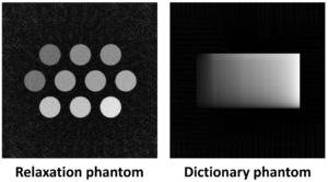
The following images are those acquired with the above sequences:

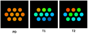
The matching results are as follows:

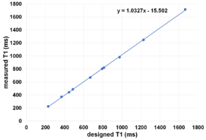
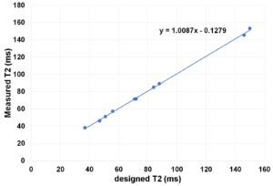
The measured relaxation times vs designed relaxation times as as follows:

 

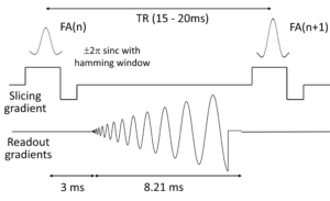
The imaging pulse sequence is as follows: